Contrastive Learning

What's Contrastive Learning

Different campuses within the same university system do not count as the sam The underlying idea of contrastive learning is to bring the distance of related samples closer and push the distance of unrelated samples farther in a certain feature space. Currently, an important issue in comparative learning is how to construct positive and negative sample pairs. In the comparative learning framework of computer vision, SimCLR, an image is expanded in two different ways to obtain a positive sample pair, while the other samples in the batch are used as negative sample pairs. In NLP, algorithms such as CLEAR propose using data augmentation methods such as random deletion, replacement, and order adjustment for data augmentation. However, due to the discreteness of the text, the text obtained through data expansion needs to be discounted in terms of text fluency and grammatical correctness. Some methods also use supervised datasets to obtain positive sample pairs, such as using questions and answers from QA datasets as a pair of positive samples. The key idea of CL is to maximize the mutual information of positive pairs. For a pair of samples and , their characteristics are and . The training objective of comparative learning can be simplified as equation:

Here , is a coefficient called temperature function. Normally, loss function can written as this norm:

The main difference of two formula is that the weight of Simple Loss for each negative sample is while contrastive learning losses result in higher penalties for negative samples with higher similarity. And temperature function pay attentions to negative samples that are hard to optimize. When tends to zero, it exert more penalties to false predictions of negative samples. Facts prove that smaller coefficient often bring benefits to performances of model.

Mutual information

In self-supervised learning, we can utilize unlabeled information in the data to train a model and learn the underlying structure and feature representations of the data. One approach involves creating auxiliary tasks by predicting certain properties of the data or by transforming the data, and then maximizing the mutual information between the predicted target and the original data. Let's consider an example where we have a dataset containing various features of houses, such as the size of the house, the number of bedrooms, the number of bathrooms, garage capacity, and their corresponding house prices. We aim to train a model that can predict house prices based on these features. We can use mutual information maximization to select the most relevant features to provide more accurate information when predicting house prices.

Assuming we have a dataset containing various features of houses, such as the size of the house, the number of bedrooms, the number of bathrooms, garage capacity, and their corresponding house prices, we want to train a model to predict house prices based on these features. We can use mutual information maximization to select the most relevant features to provide more accurate information when predicting house prices. In this specific example, we can compute the mutual information between price and size to measure their correlation. If the mutual information is high, it indicates a strong correlation between price and size, meaning that observing the price can help predict the size more accurately, or observing the size can help predict the price more accurately. The maximum mutual information is reached when there is a perfect one-to-one relationship between price and size. In other words, if we know the value of the price, the value of the size is entirely determined, and vice versa. In this case, mutual information reaches its maximum value.

Uniformity on the hypersphere

Wang et al.'s paper discussed the properties of embedded vector distribution, and they believe that an important feature of contrastive learning is its alignment and uniformity in obtaining feature vectors. As shown in Figure 3, alignment refers to similar samples having similar feature vectors, which should remain invariant to irrelevant noise. Uniformity features can store more information, meaning that the features are roughly evenly distributed on the hypersphere. Why can uniformity preserve more features? It can be understood that compared to non-uniform distributions with only a few prominent values, uniformly distributed features have a wider distribution, and each feature retains its own unique information, which can also be combined to form more results through the operation of this information.

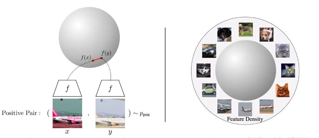
The quantification method of alignment is the expected distance between two positive sample pairs. The quantification indicator of alignment given in paper is the expected distance between positive sample pairs, as shown in equation below:

The quantitative indicator of uniformity is the radial basis function kernel (RBF kernel), represented by equation below. Among them represents the distribution of data, is a hyperparameter.

An extreme counterexample of uniformity is when the feature vectors are mapped to a point near a hypersphere, where the distribution of the feature vectors is extremely uneven. This situation is generally referred to as model collapse. Model collapse is a problem that pre training is very easy to encounter, for example, when we add some pre training tasks, it can easily lead to model collapse.

Diffences with metric learning

Contrastive learning and metric learning are both methods in the field of machine learning, used to learn the similarity and distance between data. They have some similarities, but there are also obvious differences:

Similarities:

• Objective: Both Contrastive learning and metric learning aim to learn similarity or distance measures between data points. They attempt to place similar samples in close proximity and dissimilar samples in distant locations.

• Purpose: Both methods are widely used in various machine learning tasks, such as image retrieval, facial recognition, recommendation systems, clustering, etc., to help models better understand the relationships between data.

Difference:

• Loss function:

  • Contrastive learning: Contrastive learning usually uses a Contrastive loss function, which requires the distance between similar samples to be as small as possible and the distance between dissimilar samples to be as large as possible. Common Contrastive learning methods include Siamese network, Triplet network, and recent self supervised learning methods such as Contrastive Predictive Coding (CPC) and SimCLR.

  • Metric learning: Metric learning also involves learning distance or similarity measures, but typically uses different types of loss functions, such as triplet loss or Hinge loss. Metric learning places more emphasis on learning distance metrics that are suitable for specific tasks, such as facial distance metrics in face recognition.

• Supervised：

  • Contrastive learning often use positive sample-pair generated from itself.
  • Metric learning often use positive samples-pair with the same label.

• Application field:

  • Contrastive learning: Contrastive learning is commonly used for self supervised learning and representation learning tasks, such as learning embedded representations of images, text, or audio. It is very useful in learning the representation of unlabeled data.

  • Metric learning: Metric learning is more commonly used for supervised learning tasks, especially those that require learning similarity or distance, such as face recognition, object detection, clustering, etc.

• Learning style:

  • Contrastive learning: Contrastive learning typically involves learning an embedding space where similar samples are closer in the space. It focuses on mapping data to a representation space with good properties.

  • Metric learning: Metric learning typically involves learning a distance or similarity measurement function that can be used to measure the distance or similarity between two data points. It focuses on defining a measurement function to effectively measure the relationships between data points.

In summary, both Contrastive learning and metric learning are important methods for learning the relationships between data, but their application scenarios, loss functions, and learning methods are slightly different. The choice of method depends on the nature of the task and the characteristics of the data. Sometimes, these two methods can also be combined to improve model performance.

CV：SimCLR

Contrastive Learning was used in CV field firstly. It use simple but work method to refine models' performance such as rotation image and mask some part of image, or simply let a image go through encoder twice to get a pair of positive samples.

NLP：SimCSE

SimCSE, a sentence embedding model use same methods as SimCLR did. It can work in self-supervised mode and supervisord mode.

In self-supervised mode, it generates positive sentence instance by feeding them into same encoder, but with different Drop-out to prevent label leakage(or else model will think sentence with same length are more similar).

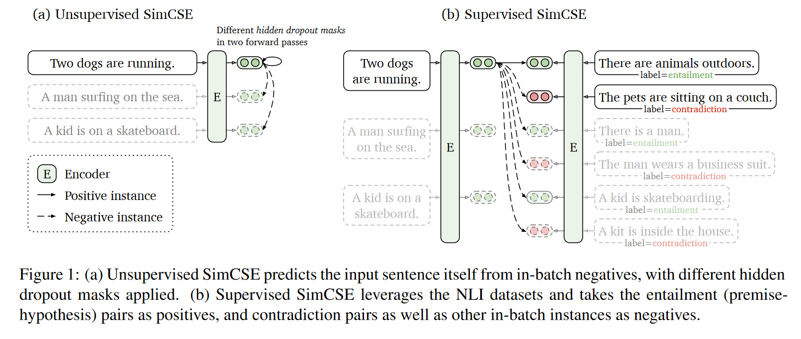
In supervised mode, it works better than bert in many field for contrastive learning greatly alleviates representation degeneration problem.

However, SimCSE still has these shortcomings:

• The sentences fed into model are identical which are only different in desperate drop-out encoders. So model may think sentences with very same length relate to same semantics.
• To overcome this shortage, there are some methods to repete some words in sentences in positive samples but not to change their meanings. And also choice some negative samples whose sentences with same length.