# Fine Tune Method

Fine-tuning is a process in machine learning, particularly in deep learning, where a pre-trained model is adapted to a new task or dataset. The goal is to leverage the knowledge learned by the model on a large dataset (often called the source domain) and apply it to a different but related task (the target domain). Here are some common fine-tuning methods in the past years:

Full Fine-Tuning: This involves training the entire model end-to-end, including the pre-trained weights. The model is updated on the new task, and all layers are allowed to learn new weights. This is suitable when the target domain is significantly different from the source domain.
Layer-Wise Pretraining: In this approach, the model is often divided into two parts: a base network and a classification layer. The base network is pre-trained on a large dataset, and the classification layer is fine-tuned on the target task. This is common in vision tasks like image classification.
Transfer Learning: This is a broader term that encompasses fine-tuning. It involves taking a model trained on one task and adapting it to another related task. The pre-trained model can be used as a starting point, and additional layers or modifications can be added to better suit the new task.
Freeze and Unfreeze: In this method, some layers of the pre-trained model are kept frozen (i.e., their weights are not updated), while others are allowed to learn new weights. This is useful when the lower layers (e.g., convolutional layers) have learned generic features that are useful for the new task, and only the higher layers (e.g., fully connected layers) need to be adapted.
Multi-Task Learning: This involves fine-tuning a model that was trained on multiple tasks simultaneously. The model learns to handle different tasks, and fine-tuning can be applied to improve performance on a specific task.
Domain Adaptation: This is a specialized form of fine-tuning where the model is adapted to perform well on a new domain. Techniques like adversarial training and domain adversarial neural networks (DANNs) are used to minimize the domain shift between the source and target domains.
Data Augmentation: While not a fine-tuning method per se, data augmentation is often used in conjunction with fine-tuning to increase the diversity of the training data and improve the model's ability to generalize.
Scheduled Sampling: This technique involves periodically sampling from the pre-trained model's output during fine-tuning, which can help prevent overfitting and improve generalization.
Model Pruning: In some cases, fine-tuning involves pruning the pre-trained model, removing less important weights or entire layers, and then training the reduced model on the new task.

These methods can be combined or modified based on the specific requirements of the target task and the differences between the source and target domains. The choice of fine-tuning method can significantly impact the performance of the adapted model.

Below are some SOTA methods to fine tuning LLM.

# LoRA

The implementation process of LoRA is as follows:

Add a bypass alongside the original pre-trained language model (PLM), perform a dimensionality reduction followed by an upscaling operation to simulate the so-called intrinsic rank.
During training, fix the parameters of the PLM and only train the dimensionality reduction matrix and the upscaling matrix .
The input and output dimensions of the model remain unchanged, and at the output, the BA is added to the parameters of the PLM.
Initialize with a random Gaussian distribution and initialize with a zero matrix, ensuring that the bypass matrix remains a zero matrix at the beginning of the training.

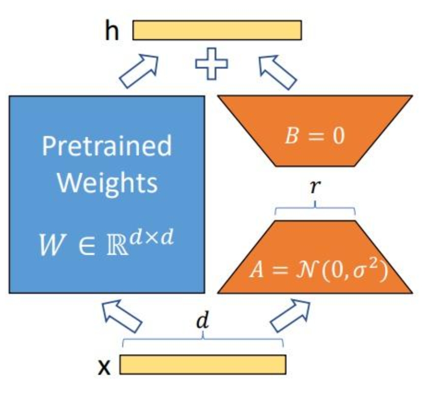
Next, we will explain the implementation of LoRA from a formulaic perspective. Assuming you want to fine-tune a pre-trained language model (such as GPT-3) for a downstream task, the need arises to update the parameters of the pre-trained model, which can be represented by the following formula:

represents the parameters initialized in the pre-trained model, and ΔW represents the parameters that need to be updated. If full parameter fine-tuning is performed, its parameter volume equals the volume of (for GPT-3, ΔW is approximately 175 billion). This shows that it is impossible for small-scale operations to fully fine-tune large language models.

Building on the work of predecessors, it has been discovered that pre-trained language models have a lower "intrinsic dimension." Even when randomly projected into a smaller subspace during task adaptation, they can still learn effectively. Therefore, what LoRA does is to add a small parameter module to learn the change .

During the training process, remains fixed and unchanged, while only the matrices and contain the trainable parameters and are subject to change.

In the inference process, there is no delay as the change is simply reintegrated back into the original model.

If you wish to switch tasks, during the task-switching process, you subtract and then replace it with $BA￥ that has been trained for another task.

# Intuition

Large models possess the concept of intrinsic dimensionality, which means that only a small number of parameters need to be adjusted to achieve good performance on downstream tasks.

For a model with a parameter count of , training it implies searching for an effective solution within a -dimensional space. However, might be redundant, and it may be possible to find an effective solution by optimizing only parameters out of the total, where is less than .

In summary, leveraging the intrinsic low-rank nature of large models, LoRA adds a bypass matrix to simulate full fine-tuning, making it a simple and effective solution for lightweight fine-tuning. This technology has been widely applied in the fine-tuning of large models, such as Alpaca, stable diffusion with LoRA, and it can be effectively combined with other parameter-efficient fine-tuning methods, such as State-of-the-art Parameter-Efficient Fine-Tuning (PEFT).

# QLoRA

LoRA is already quite impressive, but fine-tuning large models like LLaMA-65b can still be quite challenging, as loading a 65 billion-parameter model into the GPU is no small feat. QLoRA introduces a series of measures to further reduce GPU memory consumption, the most significant of which is quantizing the base model during the fine-tuning process, which further reduces the GPU memory usage caused by the number of parameters. The paper also found that the errors introduced by quantization can be eliminated during the fine-tuning process. As a result, QLoRA has become the most efficient fine-tuning solution for large language models (LLMs) to date.

QLoRA (Quantized Low-Rank Adaptation) is an adaptation of the LoRA (Low-Rank Adaptation) technique, which is designed to fine-tune large language models (LLMs) efficiently. QLoRA introduces quantization to the low-rank matrices used in LoRA, aiming to further reduce computational costs and memory usage while maintaining performance. Here are the key implementation details and technical aspects of QLoRA:

Quantization: QLoRA applies quantization to the low-rank matrices that are injected into the model. This process reduces the precision of the model's parameters, which can lead to smaller model sizes and faster training times. Quantization is typically done to a lower bit-width, such as 8-bit or 16-bit, compared to the standard 32-bit floating-point precision.
Adaptation Process: Similar to LoRA, QLoRA adapts the pre-trained model's weights by adding low-rank matrices that are applied to the model's layers. These matrices are trained to adjust the model's behavior for the target task, while the majority of the model's weights remain frozen.
Memory and Computational Efficiency: By using quantized low-rank matrices, QLoRA reduces the memory footprint and computational complexity of the fine-tuning process. This is particularly beneficial for models with billions of parameters, where full fine-tuning can be prohibitively expensive.
Training: The quantized low-rank matrices are trained alongside the pre-trained model, with the goal of minimizing the difference between the adapted model's output and the target task's desired output. The training process is typically done using gradient descent with backpropagation, just like in standard fine-tuning.
Main Differences from LoRA: The primary distinction between QLoRA and LoRA is the use of quantization. While LoRA uses full-precision floating-point numbers for the low-rank matrices, QLoRA uses lower precision, which can lead to faster training and inference times, albeit with a potential trade-off in model accuracy.
Performance: QLoRA aims to achieve performance comparable to full fine-tuning while using significantly fewer parameters. This makes it an attractive option for tasks where full fine-tuning is not feasible due to computational constraints.

# QALoRA

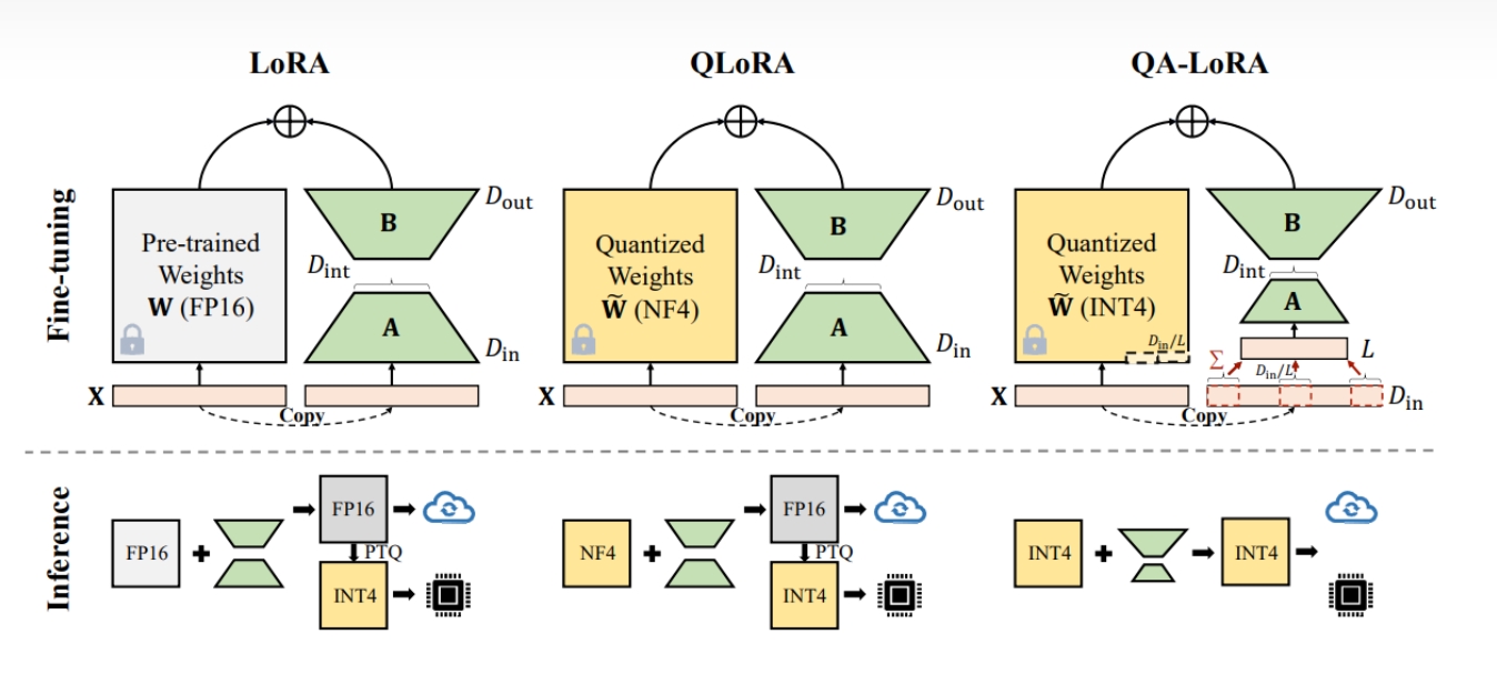
QA-LoRA aims to achieve two objectives. First, during the fine-tuning stage, the pre-trained weights are quantized to a low-bit representation, enabling LLMs to be fine-tuned on as few GPUs as possible. Second, after the fine-tuning stage, the weights that have been fine-tuned and merged remain in a quantized form, allowing LLMs to be deployed with computational efficiency.

# The main objective is twofold:

During fine-tuning, the pretrained weights are converted to a low-bit format to allow LLMs to be fine-tuned using minimal GPUs.
Post fine-tuning, the adjusted and combined weights remain in a quantized format for efficient LLM deployment.

QLoRA, a recent LoRA variant, achieved the first goal by quantizing W from FP16 to NF4 during fine-tuning. This joint optimization of quantization and adaptation is feasible as the accuracy difference between and is offset by the low-rank weights . However, after fine-tuning, the side weights are reintegrated to W~, reverting the final weights W' to FP16. Post-training quantization on W' can lead to notable accuracy loss, especially with a low bit width. Moreover, there’s no current optimization for NF4, hindering acceleration during fine-tuning and inference. Thus, QLoRA’s primary advantage is reducing memory usage during fine-tuning.

# Solution: group-wise quantization with low-rank adaptation

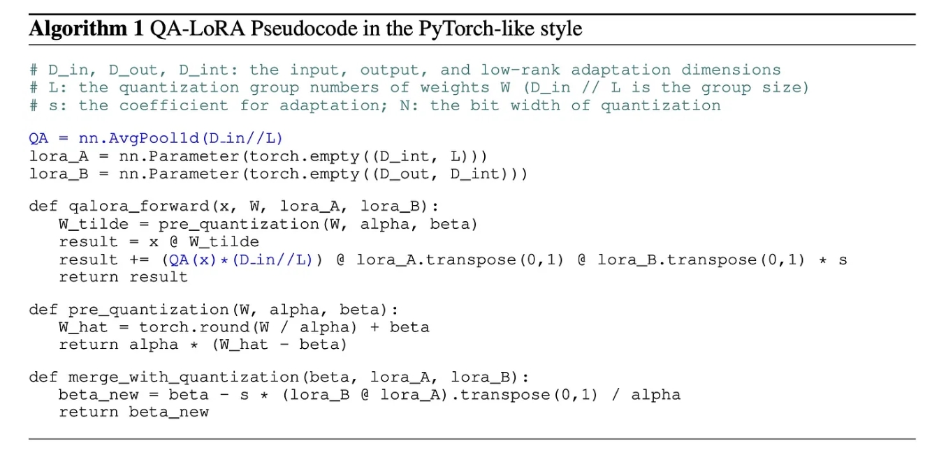
The primary objective is to merge the quantized and without resorting to high-precision numbers like FP16. In the original setting, this is unattainable due to the column-wise quantization of W and the unconstrained nature of matrices A and B. The first idea of the authors requires all row vectors of A to be identical. However, this approach results in a significant accuracy drop since it limits the rank of AB to 1, affecting the fine-tuning ability.

To address this, the constraints for both quantization and adaptation are relaxed. W is partitioned into L groups, and individual scaling and zero factors are used for quantization within each group. This also requires row vectors of A within the same group to be identical. The approach requires with minimal code changes. Compared to LoRA and QLoRA, QA-LoRA offers time and memory benefits. It requires extra storage for scaling and zero factors but reduces the parameters of A.

# Adapter

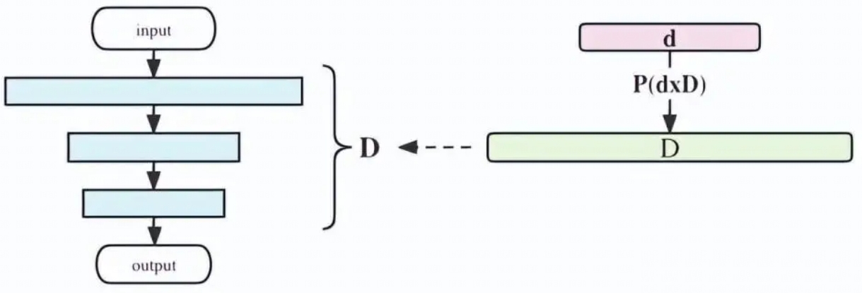
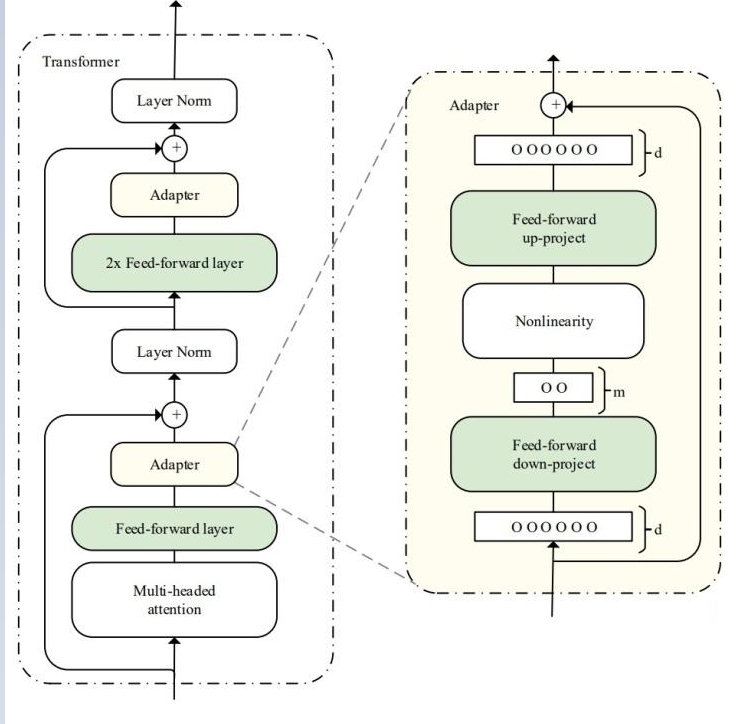
In the pre-trained model, Adapter modules (as shown in the structure on the left side of the figure) are added to each layer (or certain layers), and during fine-tuning, the main body of the pre-trained model is frozen, with the Adapter modules learning knowledge specific to the downstream task. Each Adapter module consists of two feedforward sub-layers. The first feedforward sub-layer takes the output of the Transformer block as input and projects the original input dimension d to m, controlling the size of m to limit the parameter count of the Adapter module, typically with m << d. In the output stage, the input dimension is restored through the second feedforward sub-layer, projecting m back to d as the output of the Adapter module (as shown in the structure on the right side of the figure). By adding Adapter modules, an easily scalable downstream model is created. Whenever a new downstream task arises, Adapter modules are added to avoid the issues of full model fine-tuning and catastrophic forgetting. The Adapter method does not require fine-tuning all parameters of the pre-trained model. Instead, it introduces a small number of parameters specific to the task to store knowledge about that task, reducing the computational power required for model fine-tuning.

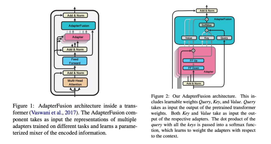
AdapterFusion divides the learning process into two stages:

Knowledge Extraction Phase: Train Adapter modules to learn specific knowledge for downstream tasks, encapsulating this knowledge within the parameters of the Adapter modules.
Knowledge Composition Phase: Fix the pre-trained model parameters Θ and the task-specific Adapter parameters Φ, introduce new parameters Ψ, and train with datasets from N downstream tasks, allowing AdapterFusion to learn how to combine the knowledge from N adapters to solve specific tasks. Parameters Ψ include Key, Value, and Query for each layer (as shown in the architecture on the right side of the figure). In each layer of the Transformer, the output of the feedforward network sub-layer serves as the Query, and the Value and Key inputs are the outputs of their respective adapters. The Query and Key are multiplied and passed into the SoftMax function, where AdapterFusion learns to weight the adapters based on the context. In a given context, AdapterFusion learns the parameter mixture of the trained adapters, identifying and activating the most useful adapters based on the given input.

The authors address the issues of catastrophic forgetting, task interference, and training instability by dividing the training of adapters into knowledge extraction and knowledge composition. The addition of Adapter modules also leads to an increase in the overall parameter count of the model, which can reduce the model's performance during inference.

Adapter Fusion optimizes the Adapter approach by dividing the learning process into two stages to enhance performance on downstream tasks. The authors compare and contrast the performance of full model fine-tuning (Full), Adapter, and AdapterFusion across various datasets. AdapterFusion outperforms full model fine-tuning and Adapter in most cases, especially on MRPC (a dataset for similarity and entailment tasks) and RTE (a dataset for recognizing text entailment), where its performance is significantly better than the other two methods.

# Prefix-tuning

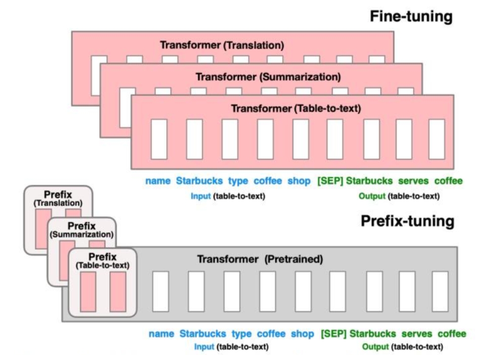
Prefix-tuning is a technique for fine-tuning large language models (LLMs) that involves adding a small set of "prefix" parameters to the model, which are specific to a particular task. This method aims to improve the model's performance on a given task without the need for full parameter fine-tuning, which can be computationally expensive and resource-intensive.

The concept of prefix-tuning was introduced to address the limitations of full parameter fine-tuning, where the entire model is updated with task-specific data. Prefix-tuning, on the other hand, only updates a small subset of parameters that are added as a prefix to the input text. These prefix parameters are designed to guide the model's behavior for the specific task at hand.

Introduction of Prefix Parameters: In prefix-tuning, a few parameters are added to the beginning of the input sequence. These parameters, often referred to as "prefix tokens," are specific to the task and are used to provide context or instructions to the model.
Task-Specific Guidance: The prefix tokens serve as a form of task-specific guidance, similar to how a human might be given instructions before performing a task. For example, in a translation task, the prefix might include the word "Translate" followed by the source language and the text to be translated.
Model Training: During training, the model learns to adjust its output based on the prefix tokens. The rest of the model's parameters remain frozen, and only the prefix parameters are updated.
Efficiency: Prefix-tuning is efficient because it requires training only a small number of parameters compared to full fine-tuning. This makes it suitable for tasks with limited data or when computational resources are scarce.
Performance: Studies have shown that prefix-tuning can achieve comparable performance to full fine-tuning on certain tasks, especially in low-data settings or when dealing with unseen topics.
Challenges: Despite its efficiency, prefix-tuning may not always outperform full fine-tuning, particularly on more complex tasks or when the model needs to learn more nuanced behaviors specific to the task.

# P-tuning

P-tuning, also known as Prompt Tuning, is a technique for fine-tuning large language models (LLMs) that involves the use of prompts to guide the model's behavior. It is a form of prompt engineering that aims to improve the model's performance on specific tasks by providing it with additional context or instructions through carefully crafted input text.

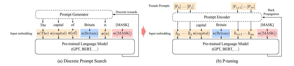
P-Tuning, as described in the paper "GPT Understands, Too" (2021), is an innovative approach to fine-tuning large language models (LLMs) that focuses on the use of prompts to guide the model's behavior. The method aims to overcome the limitations of traditional prompt-based fine-tuning, which can sometimes lead to suboptimal performance due to the discrete nature of the prompts and the potential for the model to get stuck in local optima.

Prompt Embedding: In P-Tuning, prompts are converted into learnable embedding layers. This is a departure from the typical approach of using fixed, discrete tokens as prompts, which can be problematic for continuous models like GPT.
Prompt Encoder: To address the issue of local optima, the authors propose using a prompt encoder, which consists of a multilayer perceptron (MLP) followed by a long short-term memory (LSTM) network. This encoder is trained to generate continuous prompt embeddings that are more flexible and can better capture the nuances of the task at hand.
Training Process: During training, the prompt encoder is used to generate prompt embeddings that are then concatenated with the input tokens. These combined embeddings are fed into the pre-trained language model, which is fine-tuned on the task-specific data.
Advantages:
Continuous Representation: By using a continuous representation for prompts, P-Tuning allows for smoother gradients and potentially better optimization.
Reduced Local Optima: The prompt encoder helps to avoid getting stuck in local optima by generating embeddings that are more closely related to the task requirements.
Improved Performance: The authors demonstrate that P-Tuning can achieve results comparable to full fine-tuning, especially for smaller models and on tasks where the model's architecture is not fully utilized.

← Program type Variable Auto Encoder →