# Dynamic Graph

# Type

Temporal graphs, which describe graph structures that evolve over time, can be interpreted in several ways, mainly depending on how the data is represented and processed. Here are some common interpretations of temporal graphs:

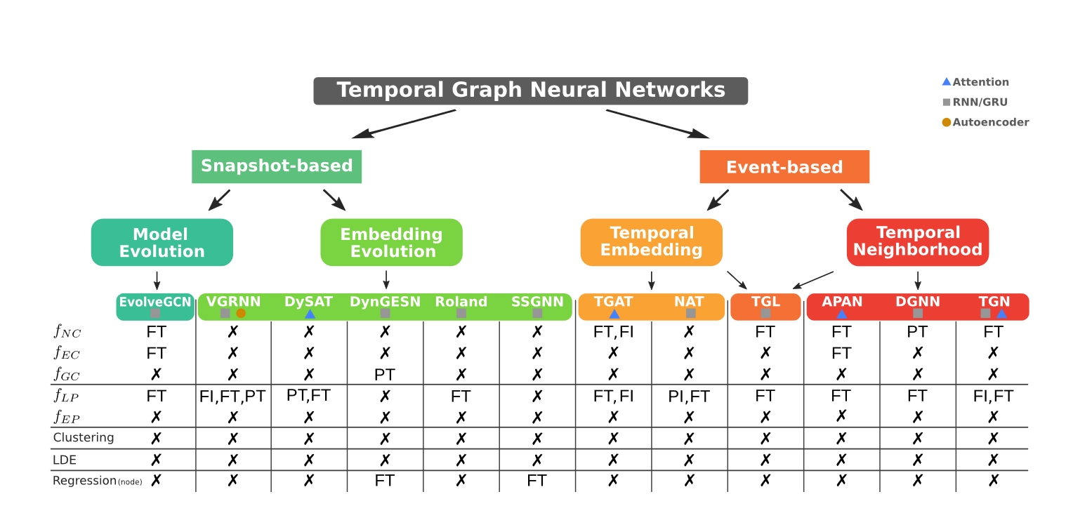
Snapshot-based Temporal Graphs (STGs):This representation breaks down the temporal graph into a series of static graph snapshots, each representing the state of the graph at a specific point in time. This method is convenient for analyzing structural changes in the graph but may not capture the dynamic evolution between consecutive time points as effectively.
Event-based Temporal Graphs (ETGs):ETGs represent the dynamic changes in the graph by recording the insertion and deletion events of nodes and edges. This approach can capture the evolution of the graph in finer detail but may require more complex data processing and analysis techniques.
Discrete Time Temporal Graphs (DTTGs):In this representation, time is divided into fixed intervals, with each interval representing a time step. The state of the graph at each time step is recorded as a snapshot. This method is suitable for scenarios where the time step size is fixed and the changes are regular, but it may not be as flexible for more irregular or rapid changes.
Continuous Time Temporal Graphs (CTTGs):Unlike DTTGs, CTTGs allow timestamps to vary continuously along a time axis, which enables the representation of more nuanced temporal changes. However, this also means that the data may be sparser and potentially more complex to handle.
Dynamic Graphs:The term "dynamic graphs" is a broader concept that encompasses all forms of temporal graphs, emphasizing the changes in graph elements (nodes and edges) over time. Dynamic graphs can be snapshot-based, event-based, discrete-time, or continuous-time, depending on the specific application and analysis objectives.

Each interpretation has its strengths and limitations, and the choice of which method to use depends on the specific application scenario and the goals of the analysis. For instance, event-based representations might be more suitable for systems with rapid changes, while snapshot-based representations could be more convenient for analyzing long-term trends.

# Task

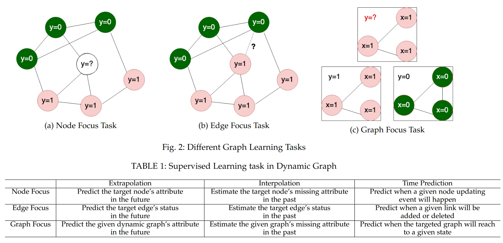
On temporal graphs, several types of tasks are commonly perform:

Node Classification: Predict the category labels for each node in the graph. This can involve predicting future states of nodes (future prediction) or inferring past states of nodes (past prediction).
Link Prediction: Predict the presence of future edges (edge prediction) or recovering past edges (edge recovery) in the graph.
Graph Classification: Classify the entire graph into different categories, such as healthy networks versus disease networks.
Event Time Prediction: Predict the time at which specific events (such as node insertions or deletions) occur in the graph.
Node Clustering: Group nodes in the graph based on their attributes and/or interactions over time.
Graph Clustering: Group a collection of temporal graphs based on their structural and/or content features.
Low-dimensional Embedding: Learn to map nodes or graphs into a low-dimensional space for visualization, similarity analysis, or further machine learning tasks.
Graph Generation: Generate new temporal graphs, either as extensions of existing graph structures or as entirely new graph structures.
Temporal Graph Analysis: Analyze the dynamic characteristics of temporal graphs, such as the evolution patterns of nodes and edges, and the changes in community structures.
Temporal Graph Visualization: Display the structure and temporal changes of temporal graphs using visualization techniques.

These tasks can be applied across various domains, such as social network analysis, traffic flow prediction, disease spread modeling, recommendation systems, and more. Temporal graph learning tasks typically require consideration of the temporal dimension, which presents additional challenges for model design and training.

# Method

Temporal graphs, which describe graph structures that evolve over time, can be interpreted in several ways, and each interpretation comes with its own set of tasks and corresponding solutions:

Snapshot-based Temporal Graphs (STGs):
- Tasks: Node classification, link prediction, graph classification.
- Solutions: Use graph convolutional networks (GCNs) to learn node features on each snapshot, then aggregate features across adjacent snapshots to capture temporal dynamics. For example, recurrent neural networks (RNNs) or long short-term memory networks (LSTMs) can be used to update node embeddings.
Event-based Temporal Graphs (ETGs):
- Tasks: Node classification, link prediction, event time prediction.
- Solutions: Update node and edge representations based on event-driven methods. For instance, maintaining a "mailbox" for each node to store event information related to that node, and then updating the node's representation based on this information.
Discrete Time Temporal Graphs (DTTGs):
- Tasks: Link prediction, graph classification.
- Solutions: Apply learning methods for static graphs, such as GCNs or graph attention networks (GATs), at each discrete time step, considering dependencies between time steps. Time encoding (e.g., using time embeddings) can be used to capture temporal sequence information.
Continuous Time Temporal Graphs (CTTGs):
- Tasks: Node classification, link prediction, graph classification.
- Solutions: Use methods that can handle continuous time information, such as recurrent neural networks (RNNs) or long short-term memory networks (LSTMs), to learn dynamic representations of nodes and edges. These models can capture temporal continuity, suitable for scenarios with irregular time changes.
Dynamic Graphs:
- Tasks: Node classification, link prediction, graph classification, event time prediction, node embedding, graph embedding.
- Solutions: Choose appropriate methods based on the specific type of dynamic graph. For example, for dynamic graphs, combine snapshot and event information, using GCNs and RNNs to learn node and edge representations, and apply time series analysis techniques to handle temporal dynamics.

Each type of temporal graph presents its own challenges, such as handling large-scale data, capturing long-term dependencies, and maintaining model interpretability. Addressing these issues typically requires a combination of deep learning, graph theory, and time series analysis techniques.

# Learning Method

In the context of past prediction and future prediction, the differences between Transductive (Inductive) Learning and Inductive (Deductive) Learning are primarily reflected in the model's access to training and testing data.

Past Prediction:
- Transductive Learning: In the setting of past prediction, transductive learning implies that the model has access to all nodes and edges in the training set, including those that need to be predicted at test time. This setup allows the model to leverage all available information to make predictions, including the historical information of nodes and edges that will only be observed at test time.
- Inductive Learning: In the setting of past prediction, inductive learning is typically not applicable because inductive learning usually means the model cannot access the test set data during training. However, in the context of temporal graphs, if the model needs to predict the state of nodes at past time points that are unknown at training time, this can be considered a special case of inductive learning, specifically past inductive learning.
Future Prediction:
- Transductive Learning: In the setting of future prediction, transductive learning means that the model has access to all nodes and edges in the training set, and these nodes and edges are also visible at test time. The model uses this information to predict the state of nodes or the properties of the graph at future time points.
- Inductive Learning: In the setting of future prediction, inductive learning means that the model can only access a subset of nodes and edges during training, and the nodes and edges at test time are unknown at training time. The model must learn to make predictions from data it has never seen before, which typically involves predicting the state of nodes or the properties of the graph at unobserved future time points.

# Time Feature

# Explicit Time Learning:

Explicit time learning algorithms use time as an independent feature input to the model. This means that the model is directly provided with information about the timestamps or time intervals associated with the graph data. These algorithms are capable of recognizing temporal patterns, such as periodicity and vector clocks, which are phenomena related to the timing of events in the graph. Explicit time learning allows for tasks like time prediction, where the model predicts when a specific event will occur in the future. This is not possible with implicit time learning methods. Examples of explicit time learning algorithms include Temporal Graph Attention Network (TGAT) and Temporal Graph Neural Network (TGN), which use Time2Vec encoding to represent time as a vector and incorporate it into the learning process.

# Implicit Time Learning:

Implicit time learning algorithms do not explicitly use time as an input feature. Instead, they rely on the ordering of the graph snapshots or the sequential nature of the data to infer temporal information. These models learn temporal patterns indirectly through the sequence of graph snapshots or updates, without the need for explicit time stamps. Implicit time learning is less capable of capturing complex temporal dynamics compared to explicit time learning, as it does not directly model the time dimension. Examples of implicit time learning include methods that use Recurrent Neural Networks (RNNs) or Long Short-Term Memory (LSTM) networks as decoders to learn temporal correlations from the sequence of graph snapshots.

# Discrete Time Dynamic Graphs (DTDG) and Continuous Time Dynamic Graphs (CTDG)

# Discrete Time Dynamic Graphs (DTDG)

DTDG models represent a dynamic graph as a series of snapshots taken at discrete time intervals. Each snapshot captures the state of the graph at a specific point in time. These models are suitable for scenarios where the graph evolves in a predictable and regular manner, and the frequency of updates is consistent. DTDGs are typically stored as a list of graph observations, each associated with a timestamp, and they can lose some temporal information if the observation frequency is not set appropriately. Learning algorithms for DTDGs often use static graph encoders to generate embeddings for each snapshot and then pass these embeddings to a sequential decoder for inference.

# Continuous Time Dynamic Graphs (CTDG)

CTDG models represent a dynamic graph as a stream of graph updating events, capturing all changes and their timestamps as they occur. These models are more memory-efficient for graphs with frequent updates and can capture all temporal information, making them suitable for graphs with complex and irregular update patterns. CTDGs are stored as a collection of timestamped graph updating events, which can include node updates, edge updates, or both. Learning algorithms for CTDGs typically use dynamic graph encoders that process the stream of events and generate node-wise embeddings that capture the temporal evolution of the graph.

← GNN for Recommendation Few-shot learning in Graph →